Introduction to Autograd

This tutorial gives a brief overview of Variable and Functions, the core components Flashlight’s automatic differentiation system. We recommend reading numpy’s Tutorial or ArrayFire’s Getting Started section before starting this tutorial so that you are familiar with Flashlight’s flavor of Tensor computation.

Variable

Variable is a wrapper around an Flashlight Tensor. Flashlight’s automatic differentiation system works with Variable directly.

auto A = fl::Variable(
  fl::arange({2, 3}, 1, fl::dtype::f32)), true /* isCalcGrad */);
// get the underlying tensor from a Variable
std::cout << "A" << A.tensor() << std::endl;
// A
// [2 3 1 1]
//    0.0000     0.0000     0.0000
//    1.0000     1.0000     1.0000
std::cout << A.shape() // dimension of the Variable
// 2 3 1 1
std::cout << A.elements() // number of elements in the Variable
// 6
std::cout << A.type() // type of the Variable
// 0 <- corresponds to float32 enum

The second parameter to Variable’s constructor (isCalcGrad) specifies whether we want to compute the gradient for a Variable.

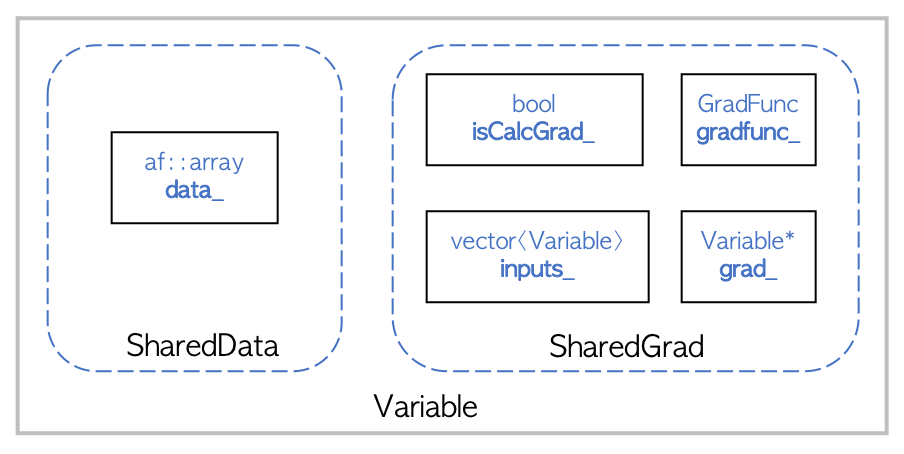
The figure above details the high-level design of Variable. SharedData and SharedGrad are shared pointer members of Variable. SharedData points to the underlying Flashlight Tensor, while SharedGrad stores gradients with respect to other Variable. The additional members facilitate a simple differentiation API which is discussed in the following sections.

It should be noted that copying a Variable creates a shallow copy; both objects will still refer to the same underlying Flashlight Tensor.

auto a = fl::Variable(fl::rand({10, 10}), false /* isCalcGrad */);
auto b = a; // shallow copy!
a.tensor() = fl::full({3, 2}, 2.0);
std::cout << "b" << b.tensor() << std::endl; // The Tensor wrapped the variable 'b' is also modified
b
[3 2 1 1]
    2.0000     2.0000
    2.0000     2.0000
    2.0000     2.0000

Complete documentation for the Variable API can be found here.

Functions

Similar to Flashlight Tensors, Variable can be used to perform Tensor operations directly.

auto var = fl::Variable(
  fl::arange({2, 3}, 1, fl::dtype::f32), true /* isCalcGrad */);
auto expVar = exp(var);
std::cout << "expVar" << expVar.tensor() << std::endl;;
// expVar
// [2 3 1 1]
//    1.0000     1.0000     1.0000
//    2.7183     2.7183     2.7183

auto A = fl::Variable(fl::full({2, 3}, 1.0), true /* isCalcGrad */);
auto B = fl::Variable(fl::full({2, 3}, 2.0), false /* isCalcGrad */);
auto AB = A * B;
std::cout << "AB" << AB.tensor() << std::endl;
// AB
// [2 3 1 1]
//    2.0000     2.0000     2.0000
//    2.0000     2.0000     2.0000

A complete list of functions can be found here.

Automatic Differentiation

Given a Variable in a computation graph with some input dependencies, if at least one of its inputs requires a gradient, each preceeding Variable in the graph must keep track of its inputs, and a method by which to compute its gradient. The latter is accomplished via gradFunc, a lambda function that takes the gradient of a Variable’s outputs and computes the gradient with respect to its inputs.

To recursively compute the gradient of a Variable with respect to all of its inputs in the computation graph, we call the backward() function on the Variable. This iteratively computes the gradients for each Variable through the computational graph using a topological ordering by repeatedly applying the chain rule. For instance, given some Variable expVar with some input Variable var, calling expVar.backward() computes the gradient of expVar with respect to var.

expVar.backward();
// expVar.grad() and varGrad are Variables
std::cout << "expVarGrad" << expVar.grad().tensor() << std::endl;
std::cout << "varGrad" << var.grad().tensor() << std::endl;
// expVarGrad
// [2 3 1 1]
//     1.0000     1.0000     1.0000
//     1.0000     1.0000     1.0000

// varGrad
// [2 3 1 1]
//     1.0000     1.0000     1.0000
//     2.7183     2.7183     2.7183

AB.backward();
std::cout << "ABGrad" << AB.grad().tensor() << std::endl;
std::cout << "AGrad" << A.grad().tensor() << std::endl;
// ABGrad
// [2 3 1 1]
//     1.0000     1.0000     1.0000
//     1.0000     1.0000     1.0000

// AGrad
// [2 3 1 1]
//     2.0000     2.0000     2.0000
//     2.0000     2.0000     2.0000

Warning

Calling B.grad() will throw an exception here since isCalcGrad is set to false

TODO: Add step-by-step execution details on an example computation graph

Various Optimizations

ArrayFire’s JIT Compiler

Note

This section is only applicable if using Flashlight’s ArrayFire backend.

ArrayFire uses a JIT compiler to combine many small function calls into a single kernel call. Below is a simple example:

auto A = fl::Variable(
    fl::rand({1000, 1000}), true); // 'A' is allocated, Total Memory: 4 MB
auto B = 2.0 * A; // 'B' is not allocated, Total Memory : 4 MB
auto C = 1.0 + B; // 'C' is not allocated, Total Memory :  4 MB
auto D = log(C); // 'D' is not allocated (yet), Total Memory :  4 MB
fl::eval(D); // only 'D' is allocated, Total Memory : 8 MB

The JIT both improves performance and reduces memory usage. For further documentation, see docs for the ArrayFire JIT.

In-Place Operations and More with ArrayFire

Note

This section is only applicable if using Flashlight’s ArrayFire backend.

Since the flashlight uses shared_ptr semantics for storing its internal ArrayFire array, any array is automatically deleted when the Variable goes out of scope.

auto A = fl::Variable(fl::rand({1000, 1000}), false); // Total Memory: 4 MB
auto B = fl::Variable(fl::rand({1000, 1000}), false); // Total Memory: 8 MB
auto C =  fl::transpose(A); // Total Memory: 12 MB
C = fl::matmul(C, fl::transpose(B)); // Total Memory: 12 MB. Previous 'C' goes out of scope

We have carefully optimized memory usage for forward and backward passes over the computation graph. Some autograd functions do not need to keep their input data after the forwad pass in order to compute their gradient during the backward pass (e.g. sum (+), transpose). For these operations, the resulting Variable need not store its input Variables’ SharedData; thus, the underlying array can be freed, as it is not referenced elsewhere.

// Note calcGrad is set to true here. Total Memory: 4 MB
auto A = fl::Variable(fl::rand({1000, 1000}), true);

// Intermediate arrays are not stored. Total Memory: 8 MB
auto C =  fl::transpose(fl::transpose(A));

Retaining the Computation Graph

The backward() function takes an additional boolean parameter, retainGraph, which is false by default. When the argument is false, each Variable that is not required is cleared from the computation graph while the backard pass is being computed as soon as it is no longer depended upon in the graph. This reduces peak memory usage while computing gradients. Setting retainGraph to true is not recommended unless intermediate values in the backward graph must be inspected.

auto A = fl::Variable(fl::rand({1000, 1000}), true);
auto B = fl::Variable(fl::rand({1000, 1000}), true);
auto C = fl::matmul(A, B);
C = fl::transpose(C);
C = 1.0 + C;
C.backward(false); // Note `retainGraph` is false by default

For example, in the above graph, the intermediate Variable E can be deleted as soon as the gradients of D are computed.